노트북 16 — LLL 기저 축소

목표: “좋은 기저”가 무엇인지 이해하고, 정의에서 출발해 LLL을 직접 구현하며, 왜곡된 기저가 거의 직교하는 기저로 변환되는 과정을 확인합니다. 순수 Python 구현입니다.

import numpy as np
import matplotlib.pyplot as plt
from pqc_edu.attacks_advanced.lll import gram_schmidt, lll_reduce

좋은 기저 vs 나쁜 기저

기저는 격자를 생성하는 벡터들의 집합입니다. 같은 격자를 생성하는 두 기저가 극단적으로 달라 보일 수 있습니다. “좋은” 기저는 짧고 거의 직교하는 벡터로 이루어져 있습니다. “나쁜” 기저는 길고 기울어진 벡터로 이루어져 있습니다. LLL은 다항 시간 안에 나쁜 것을 좋은 것으로 바꿉니다.

B = np.array([[19, 2], [12, 15]], dtype=np.int64)
R = lll_reduce(B, delta=0.99)

fig, axes = plt.subplots(1, 2, figsize=(10, 5))
for ax, basis, title in zip(axes, [B, R], ["before LLL", "after LLL"]):
    pts = []
    for i in range(-3, 4):
        for j in range(-3, 4):
            pts.append(i * basis[0] + j * basis[1])
    pts = np.array(pts)
    ax.scatter(pts[:, 0], pts[:, 1], s=8, color="steelblue", alpha=0.4)
    for v, c in zip(basis, ("red", "green")):
        ax.annotate("", xy=v, xytext=(0, 0), arrowprops=dict(arrowstyle="->", color=c, lw=2))
    ax.set_title(title)
    ax.set_aspect("equal")
    ax.axhline(0, color="lightgray", lw=0.5)
    ax.axvline(0, color="lightgray", lw=0.5)
plt.tight_layout(); plt.show()
print('before:', B.tolist())
print('after: ', R.tolist())

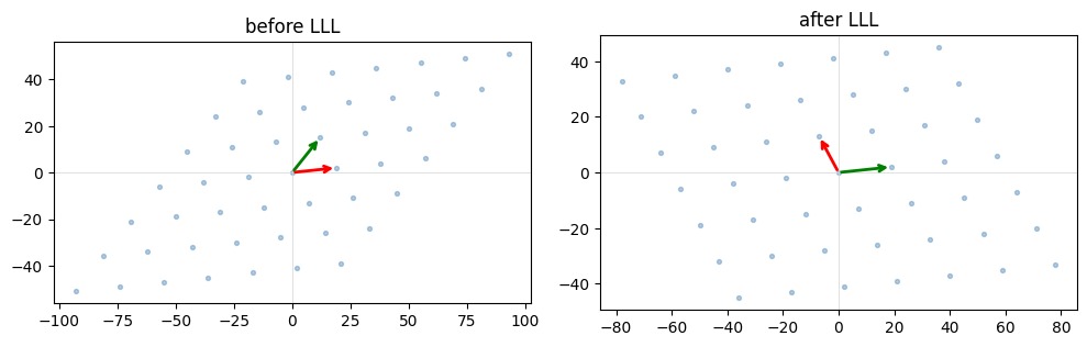
before: [[19, 2], [12, 15]]
after:  [[-7, 13], [19, 2]]

Gram-Schmidt: 직교하는 뼈대

LLL은 기저의 Gram-Schmidt 직교화(GSO)를 추적하면서 동작합니다. GSO는 이전 벡터들에 대한 projection을 빼 나가는 방식으로 직교 벡터 \(b^*_i\)를 만듭니다.

B = np.array([[4, 1, 0], [2, 2, 0], [0, 1, 3]], dtype=np.int64)
B_star, mu = gram_schmidt(B)
print('B_star:'); print(B_star)
print('\northogonal?  (dot products)')
for i in range(3):
    for j in range(i+1, 3):
        print(f'  <b*{i}, b*{j}> = {np.dot(B_star[i], B_star[j]):.2e}')

B_star:
[[ 4.00000000e+00  1.00000000e+00  0.00000000e+00]
 [-3.52941176e-01  1.41176471e+00  0.00000000e+00]
 [ 8.32667268e-17  0.00000000e+00  3.00000000e+00]]

orthogonal?  (dot products)
  <b*0, b*1> = -4.44e-16
  <b*0, b*2> = 3.33e-16
  <b*1, b*2> = -2.94e-17

LLL 조건

어떤 기저가 파라미터 \(\delta \in (1/4, 1)\)에 대해 LLL-축소(reduced)되었다는 것은 다음 두 조건이 성립한다는 뜻입니다:

1. 크기 축소(Size-reduced): 모든 \(j < i\)에 대해 \(|\mu_{i,j}| \le 1/2\).

2. Lovász: \(\|b^*_i\|^2 \ge (\delta - \mu_{i,i-1}^2)\|b^*_{i-1}\|^2\).

첫 번째는 각 벡터가 이전 벡터들과 “거의 직교”한다는 뜻입니다. 두 번째는 연속된 GSO 벡터의 길이가 너무 빨리 줄어들지 않는다는 뜻입니다.

Hermite factor — 얼마나 좋은지 측정하기

rank-\(n\) 격자 \(\Lambda\)와 determinant \(\det(\Lambda)\)가 주어졌을 때, 가장 짧은 0이 아닌 벡터 \(\lambda_1\)은 (Minkowski bound에 의해) 대략 \(\|\lambda_1\| \le \sqrt{n} \cdot \det(\Lambda)^{1/n}\)을 만족합니다.

LLL의 첫 번째 벡터는 \(\alpha = 1/(\delta - 1/4)\)에 대해 \(\|b_1\| \le \alpha^{(n-1)/2} \cdot \det(\Lambda)^{1/n}\)을 만족합니다. \(\delta = 0.99\)일 때 \(\alpha \approx 1.35\)입니다. 우리는 경험적 Hermite factor인 \(\|b_1\| / \det(\Lambda)^{1/n}\)을 측정합니다.

rng = np.random.default_rng(0)
dims = [2, 4, 6, 8, 10, 12]
factors = []
for n in dims:
    B = rng.integers(-50, 50, (n, n)).astype(np.int64)
    while abs(np.linalg.det(B)) < 1.0:
        B = rng.integers(-50, 50, (n, n)).astype(np.int64)
    R = lll_reduce(B, delta=0.99)
    det_n = abs(np.linalg.det(R.astype(float)))
    factors.append(np.linalg.norm(R[0]) / det_n ** (1.0 / n))
plt.plot(dims, factors, 'o-')
plt.xlabel('dimension n')
plt.ylabel('Hermite factor  ||b_1|| / det^(1/n)')
plt.title('Empirical Hermite factor after LLL (delta=0.99)')
plt.grid(True)
plt.show()
for n, f in zip(dims, factors):
    print(f'n={n:2d}   Hermite factor = {f:.3f}')

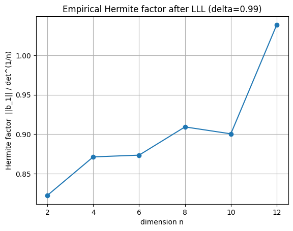
n= 2   Hermite factor = 0.822
n= 4   Hermite factor = 0.871
n= 6   Hermite factor = 0.874
n= 8   Hermite factor = 0.909
n=10   Hermite factor = 0.901
n=12   Hermite factor = 1.039

LLL이 할 수 없는 것

LLL은 근사 보장만을 제공하며, 정확한 SVP를 풀지는 못합니다. 첫 번째 벡터는 실제 최단 벡터보다 최대 \(\alpha^{(n-1)/2}\)배 길 수 있습니다. LWE를 공격하려면 LLL만으로는 부족한 정도의 짧은 벡터가 필요합니다 — 여기서 BKZ가 등장합니다.

→ 17_bkz_and_scaling.ipynb