Notebook 00c — Math toolbox

Just enough math to follow ML-KEM. Nothing abstract for its own sake.

import numpy as np

Modular arithmetic

a mod q is the remainder when a is divided by q. Throughout this book, q = 3329 (the ML-KEM prime). All arithmetic happens inside the set {0, 1, ..., q-1}.

q = 3329
print((5 + 3329) % q)        # 5
print((-1) % q)              # 3328  (note: Python's % returns non-negative)
print((2 * 1665) % q)        # 1  — 1665 is the multiplicative inverse of 2 mod 3329

5
3328
1

Why prime q? If q is prime, every nonzero element has a multiplicative inverse. This makes Z_q a field — we can add, subtract, multiply, and divide (divide = multiply by inverse). ML-KEM relies on this: without a prime q, the NTT (notebook 04) would not work.

# Modular inverse via Fermat's little theorem: a^(q-1) ≡ 1 (mod q), so a^(q-2) = a^-1.
a = 17
a_inv = pow(a, -1, q)   # Python's built-in since 3.8
print(f"{a} * {a_inv} mod {q} = {(a * a_inv) % q}")   # 1

17 * 1175 mod 3329 = 1

Vectors and matrices mod q

We will constantly use vectors in Z_q^n (length-n vectors of integers mod q) and k×k matrices of such vectors. All operations — dot product, matrix multiplication — are done modulo q.

n = 4
rng = np.random.default_rng(0)
a = rng.integers(0, q, n); s = rng.integers(0, q, n)
inner = int(a @ s) % q
print("a =", a)
print("s =", s)
print("<a, s> mod q =", inner)

A = rng.integers(0, q, (3, 3))
v = rng.integers(0, q, 3)
print("\nA =\n", A)
print("A @ v mod q =", (A @ v) % q)

a = [2831 2120 1701  898]
s = [1024  136  250   55]
<a, s> mod q = 4

A =
 [[ 583 2707 2161]
 [3038 1676 2019]
 [3231 2428 2104]]
A @ v mod q = [2841  654 1242]

Groups, rings, fields — the 30-second tour

• Group (additive): a set with an addition operation that has an identity (0) and inverses. Z_q with + mod q is a group.

• Ring: a group with an additional multiplication that distributes over addition. Z_q with +, × is a ring.

• Field: a ring where every nonzero element has a multiplicative inverse. Z_q for prime q is a field.

• ML-KEM works in R_q = Z_q[x] / (x^n + 1) — polynomials with coefficients in Z_q, reduced modulo x^n + 1. This is a ring (not a field). Notebook 04 explores it.

Hash functions and PRFs

• Hash function: deterministic, fixed-size output, collision-resistant. H(x) gives a “fingerprint.” Example: SHA-256.

• XOF (extendable-output function): like a hash, but output length is variable. ML-KEM uses SHAKE-128 and SHAKE-256.

• PRF (pseudo-random function): keyed function PRF(key, x) whose output is indistinguishable from random to anyone without the key. In ML-KEM, SHAKE-256 seeded with a secret acts as a PRF.

import hashlib
print("SHA3-256('hello') =", hashlib.sha3_256(b"hello").hexdigest())

# SHAKE-256 — variable length
h = hashlib.shake_256(); h.update(b"seed")
print("SHAKE-256 64-byte output =", h.digest(64).hex())

# Same seed → same output (deterministic)
h2 = hashlib.shake_256(); h2.update(b"seed")
print("deterministic:", h.digest(64) == h2.digest(64))

SHA3-256('hello') = 3338be694f50c5f338814986cdf0686453a888b84f424d792af4b9202398f392
SHAKE-256 64-byte output = 4fd6800b5ddf65323de29f59e5da90d3fa6778594e60e2ff4326622eff3e42c4ffb0cbd6d1735223365916ac2d97eb47b86c1573d1e640ff4f4020d805e01cd8
deterministic: True

Discrete Gaussian / small noise

Lattice crypto adds “small” noise to hide secrets. We sample from distributions concentrated near 0:

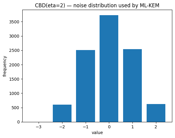
• Discrete Gaussian: round samples from N(0, σ²) to integers. Good theoretically, slightly tricky to implement in constant time.

• Centered Binomial Distribution (CBD): ML-KEM’s practical choice. Sample a, b each as η independent coin flips; output a - b. Range: {-η, ..., η}, zero-mean, symmetric, easy to sample.

rng = np.random.default_rng(0)
# CBD with eta=2: two pairs of coin flips, difference gives values in {-2, ..., 2}
eta = 2
samples = rng.integers(0, 2, (10000, 2 * eta)).sum(axis=1)
cbd = samples[:5000] - rng.integers(0, 2, (5000, 2 * eta)).sum(axis=1)
# Simpler: directly
a = rng.integers(0, 2, (10000, eta)).sum(axis=1)
b = rng.integers(0, 2, (10000, eta)).sum(axis=1)
cbd = a - b

import matplotlib.pyplot as plt
plt.hist(cbd, bins=range(-eta-1, eta+2), rwidth=0.8, align="left")
plt.title(f"CBD(eta={eta}) — noise distribution used by ML-KEM")
plt.xlabel("value"); plt.ylabel("frequency")
plt.show()

What you now have

• You can read a ≡ b (mod q), <a, s>, A·s + e, H(x), PRF(k, n) as code.

• You know why q is prime (for inverses) and what CBD looks like.

• That’s the entire math vocabulary for the rest of the book.

→ 01_lattice_intro.