Notebook 01 — What is a lattice?

Goal: build intuition for 2-D lattices and the two core hard problems — the Shortest Vector Problem (SVP) and the Closest Vector Problem (CVP).

Lattice problems are the reason post-quantum cryptography works: no known polynomial-time quantum algorithm solves them in high dimensions, even though Shor’s algorithm demolishes RSA and elliptic-curve crypto.

import numpy as np
import matplotlib.pyplot as plt
from pqc_edu.lattice import plot_lattice_2d, good_vs_bad_basis, lattice_points

Formal definition

Given a basis matrix \(B \in \mathbb{R}^{d \times d}\) whose columns are linearly independent vectors, the lattice generated by \(B\) is

\[ L(B) = \{ B z : z \in \mathbb{Z}^d \}. \]

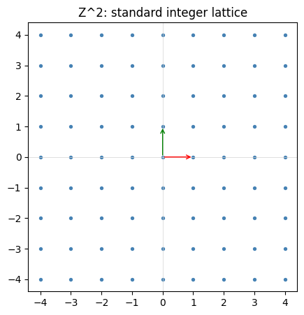
That is, the lattice is the set of all integer combinations of the basis vectors. A lattice is a discrete, infinite, regularly spaced grid of points.

plot_lattice_2d(np.eye(2), radius=4)
plt.title('Z^2: standard integer lattice')
plt.show()

Good vs. bad bases

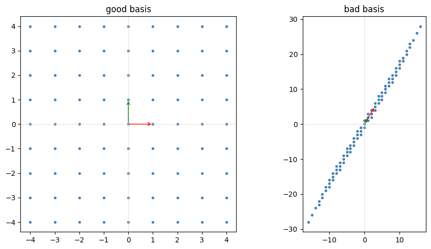
The same lattice can be described by different bases. A good basis has short, nearly orthogonal vectors. A bad basis has long, skewed vectors that are nearly parallel. Both span exactly the same set of lattice points — but algorithmically, a good basis makes CVP easy and a bad basis makes it hard. Much of lattice cryptanalysis is about turning a bad basis into a good one (lattice reduction, e.g. LLL and BKZ).

good, bad = good_vs_bad_basis()
fig, axes = plt.subplots(1, 2, figsize=(10, 5))
plot_lattice_2d(good, 4, ax=axes[0])
axes[0].set_title('good basis')
plot_lattice_2d(bad, 4, ax=axes[1])
axes[1].set_title('bad basis')
plt.tight_layout()
plt.show()

The two hard problems

Shortest Vector Problem (SVP): given a basis of \(L\), find a nonzero lattice vector of minimum Euclidean length.

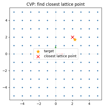
Closest Vector Problem (CVP): given a basis of \(L\) and a target point \(t \notin L\), find the lattice vector closest to \(t\).

Both problems are easy in 2-D (you can just look). In high dimensions, both are NP-hard in the worst case, and the best known algorithms — classical and quantum — take time exponential in the dimension.

target = np.array([2.3, 1.7])
plot_lattice_2d(good, 5, target=target)
plt.title('CVP: find closest lattice point')
plt.show()

Why quantum-hard?

Shor’s algorithm breaks integer factorization and the discrete logarithm in polynomial time on a quantum computer — that kills RSA, DH, and ECC.

But no known polynomial-time quantum algorithm solves approximate SVP or CVP in high dimensions. The best quantum speedups are only polynomial improvements over classical exponential-time algorithms (e.g. Grover-style).

LWE, which we meet in the next notebook, reduces to a CVP-like problem — so breaking LWE would break hard lattice problems. That’s the foundation of modern PQC (ML-KEM, ML-DSA).

→ Next: 02_toy_lwe.ipynb.