Notebook 13 — QFT and period finding

Goal: build the Quantum Fourier Transform, see it as the key to order finding, and watch it light up periodic structure as spectral peaks.

import numpy as np
import matplotlib.pyplot as plt
from pqc_edu.quantum.simulator import QuantumState, H
from pqc_edu.quantum.circuits import qft, inverse_qft, qft_matrix

The QFT in one equation

\[\text{QFT}|j\rangle = \frac{1}{\sqrt{N}} \sum_{k=0}^{N-1} e^{2\pi i jk / N} |k\rangle\]

where \(N=2^n\). Same formula as the classical Discrete Fourier Transform, just acting on amplitudes instead of samples.

print('1-qubit QFT = Hadamard?', np.allclose(qft_matrix(1), H))
print('\n2-qubit QFT matrix:')
print(np.round(qft_matrix(2), 3))

1-qubit QFT = Hadamard? True

2-qubit QFT matrix:
[[ 0.5+0.j   0.5+0.j   0.5+0.j   0.5+0.j ]
 [ 0.5+0.j   0. +0.5j -0.5+0.j  -0. -0.5j]
 [ 0.5+0.j  -0.5+0.j   0.5-0.j  -0.5+0.j ]
 [ 0.5+0.j  -0. -0.5j -0.5+0.j   0. +0.5j]]

Roundtrip: QFT then inverse-QFT gives back the input

rng = np.random.default_rng(0)
q = QuantumState(4)
q.amps = rng.standard_normal(16) + 1j*rng.standard_normal(16)
q.amps /= np.linalg.norm(q.amps)
before = q.amps.copy()
qft(q, list(range(4)))
inverse_qft(q, list(range(4)))
print('roundtrip exact:', np.allclose(q.amps, before, atol=1e-10))

roundtrip exact: True

The magic: period → peaks

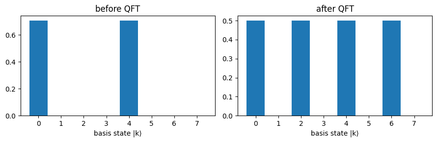
Take an 8-dim register prepared in a periodic comb: amplitude 1 at indices {0, 4} (period 4). Apply the QFT. The result should have peaks at indices that are multiples of \(N/\text{period} = 8/4 = 2\), i.e. at {0, 2, 4, 6}.

n = 3
q = QuantumState(n)
q.amps[:] = 0.0
for k in (0, 4):
    q.amps[k] = 1.0
q.amps /= np.linalg.norm(q.amps)
before = np.abs(q.amps).copy()
qft(q, list(range(n)))
after = np.abs(q.amps)

fig, axes = plt.subplots(1, 2, figsize=(9, 3))
axes[0].bar(range(8), before)
axes[0].set_title('before QFT')
axes[0].set_xlabel('basis state |k⟩')
axes[1].bar(range(8), after)
axes[1].set_title('after QFT')
axes[1].set_xlabel('basis state |k⟩')
plt.tight_layout()
plt.show()

Shor’s recipe, informally

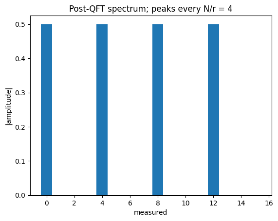
If we can prepare a superposition \(\sum_x |x\rangle|f(x)\rangle\) where \(f(x) = a^x \bmod N\), the \(y\) register will hold a periodic pattern (period = order of \(a\) mod \(N\)). Measuring it collapses to a fixed value, leaving the \(x\) register in a comb-like superposition at that period. Apply QFT to reveal peaks at multiples of \(2^n / r\) — continued fractions recover \(r\).

n = 4
q = QuantumState(n)
q.amps[:] = 0.0
period = 4
indices = list(range(0, 16, period))
for k in indices:
    q.amps[k] = 1.0
q.amps /= np.linalg.norm(q.amps)
qft(q, list(range(n)))
plt.bar(range(16), np.abs(q.amps))
plt.xlabel('measured')
plt.ylabel('|amplitude|')
plt.title(f'Post-QFT spectrum; peaks every N/r = {16//period}')
plt.show()

Next up

We now have all the pieces. Next notebook assembles them into Shor’s algorithm and watches RSA-sized toy numbers fall. → 14_shor_breaks_rsa.ipynb